Case Study

Extraction and preparation of Sepsis data for Machine Learning applications.

Outline

1. Introduction

2. Set-up

3. Cohort Selection

4. Data Standardisation

5. Data Preperation

6. Data Pre-processing

7. Data Preparation

8. Conclusion

1. Introduction

In this case study, our main objective is to showcase the effectiveness of EHR-QC by employing the toolkit to handle EHR data comprehensively and preparing it for utilisation in subsequent usage in Machine Learning. To illustrate, we select a group of patients who have been diagnosed with Sepsis from the public MIMIC IV EHR database. Subsequently, we employ the EHR-QC standardisation module to convert the raw EHR data to the OMOP-CDM schema. Following this, we employ the EHR-QC data pre-processing module. This involves extracting information from the standardised schema, generating exploratory reports, and identifying as well as rectifying any anomalies present in the data.

2. Set-up

In this case study, we utiliseed the Dockerised EHR-QC. For comprehensive instructions on configuring the Docker environment, please consult the documentation provided at the following link: https://ehr-qc-tutorials.readthedocs.io/en/latest/install.html#docker

3. Cohort selection

From the MIMIC IV dataset, we’ve identified all patients and admissions related to Sepsis. This selection involves utilising ICD-9 codes 995.91, 995.92, and 785.52, as well as ICD-10 codes A419, R6520, and R6521 which pertain to Sepsis, Severe Sepsis, and Septic Shock. Subsequently, we’ve extracted the complete EHR data associated with these patients and admissions, converting them into csv files.

This process yielded a cohort containing 12,276 patients corresponding to 14,870 admissions, along with their respective EHR data.

4. Data standardisation

In the subsequent phase, the EHR data associated with the Sepsis cohort, as contained in the CSV files, is standardised to the OMOP-CDM schema. This task is accomplished through the utilisation of the EHR-QC utility, which carries out a series of sequential steps, culminating standard EHR representation in a relational database. The information required by the code to source the data, store the intermediate data, and dump the standardised EHR are provided in the configuration file as shown below before executing the utility functions. For more details on configuration options, refer the documentation: https://ehr-qc-tutorials.readthedocs.io/en/latest/config.html

# database connection details
db_details = {
    "sql_host_name": <Host Name>,
    "sql_port_number": <Port Number>,
    "sql_user_name": <User Name>,
    "sql_password": ******,
    "sql_db_name": <DB Name>,
}

# new schema to host the migrated tables

lookup_schema_name = 'vocabulary_test_20230809'

source_schema_name = 'omop_migration_source_20230809'

etl_schema_name = 'omop_migration_etl_20230809'

cdm_schema_name = 'omop_test_20230809'

Running the standardisation involves the following stages:

1. Incorporating the Standard Vocabulary

Note

We have used Athena (https://athena.ohdsi.org/) as a source of standard vocabulary

If running via command line:

(.venv) app_user@hostname:~$python -m ehrqc.standardise.migrate_omop.Run -l

If using Jupyter notebook:

import os

os.system(
    '''cd /path/to/EHRQC;'''
    +
    '''.venv/bin/python -m ehrqc.standardise.migrate_omop.Run -l'''
    )

The paths of the files containing controlled vocabulary concepts are obtained from configuration file as shown below. For more details on configuration options, refer the documentation: https://ehr-qc-tutorials.readthedocs.io/en/latest/config.html

vocabulary = {
    'concept': '/path/to/CONCEPT.csv',
    'vocabulary': '/path/to/VOCABULARY.csv',
    'domain': '/path/to/DOMAIN.csv',
    'concept_class': '/path/to/CONCEPT_CLASS.csv',
    'concept_relationship': '/path/to/CONCEPT_RELATIONSHIP.csv',
    'relationship': '/path/to/RELATIONSHIP.csv',
    'concept_synonym': '/path/to/CONCEPT_SYNONYM.csv',
    'concept_ancestor': '/path/to/CONCEPT_ANCESTOR.csv',
    'tmp_custom_mapping': '/path/to/tmp_custom_mapping.csv',
}

2. Importing EHR data from the CSV files

If running via command line:

(.venv) app_user@hostname:~$python -m ehrqc.standardise.migrate_omop.Run -f

If using Jupyter notebook:

import os

os.system(
    '''cd /path/to/EHRQC;'''
    +
    '''.venv/bin/python -m ehrqc.standardise.migrate_omop.Run -f'''
    )

The paths and the column mapping (if other than the expected names) needs to configured in the configuration file as shown below before running this command. For more details on configuration options, refer the documentation: https://ehr-qc-tutorials.readthedocs.io/en/latest/config.html

# CSV file column mapping

patients = {
    'file_name': '/path/to/patients.csv',
    'column_mapping': {
        'subject_id': 'non_standard_subject_id',
        'gender': 'non_standard_gender',
        'anchor_age': 'non_standard_anchor_age',
        'anchor_year': 'non_standard_anchor_year',
        'anchor_year_group': 'non_standard_anchor_year_group',
        'dod': 'non_standard_dod'
    },
}

3. Staging the data within staging tables

If running via command line:

(.venv) app_user@hostname:~$python -m ehrqc.standardise.migrate_omop.Run -s

If using Jupyter notebook:

import os

os.system(
    '''cd /path/to/EHRQC;'''
    +
    '''.venv/bin/python -m ehrqc.standardise.migrate_omop.Run -s'''
    )

4. Integrating custom concept mappings for concepts that deviate from the standard

If running via command line:

(.venv) app_user@hostname:~$python -m ehrqc.standardise.migrate_omop.Run -c

If using Jupyter notebook:

import os

os.system(
    '''cd /path/to/EHRQC;'''
    +
    '''.venv/bin/python -m ehrqc.standardise.migrate_omop.Run -c'''
    )

5. Executing the migration process

If running via command line:

(.venv) app_user@hostname:~$python -m ehrqc.standardise.migrate_omop.Run -e

If using Jupyter notebook:

import os

os.system(
    '''cd /path/to/EHRQC;'''
    +
    '''.venv/bin/python -m ehrqc.standardise.migrate_omop.Run -e'''
    )

6. Transitioning to the OMOP-CDM schema

If running via command line:

(.venv) app_user@hostname:~$python -m ehrqc.standardise.migrate_omop.Run -u

If using Jupyter notebook:

import os

os.system(
    '''cd /path/to/EHRQC;'''
    +
    '''.venv/bin/python -m ehrqc.standardise.migrate_omop.Run -u'''
    )

For more comprehensive insights into each of these stages, please consult the following link: https://ehr-qc-tutorials.readthedocs.io/en/latest/migrate.html#omop-cdm-migration.

This resulted in the successful migration of the entire cohort (100 %), encompassing all the 12,276 patients and 14,870 admissions, alongside their respective EHR data in a fully automated manner.

Utilising well-established, compatible tools and techniques becomes notably more straightforward when working with data that has been transformed into a standardised format.

5. Data Extraction

During this stage, we retrieve the demographics, vital signs, and lab measurements of the Sepsis cohort from the standardised OMOP-CDM schema using EHR-QC pre-processing module.

Successful extraction using the following commands yielded;

If running via command line:

(.venv) app_user@hostname:~$python -m ehrqc.extract.Extract /save/path/demographics.csv omop demographics omop_test_20230809

If using Jupyter notebook:

import os

os.system(
    '''cd /path/to/EHRQC;'''
    +
    '''.venv/bin/python -m ehrqc.extract.Extract /save/path/demographics.csv omop demographics omop_test_20230809'''
    )

1. Demographics data for 12,276 patients, encompassing 7 attributes: Age, Weight, Height, Gender, Ethnicity, Date of Birth, and Date of Death (if applicable)

If running via command line:

(.venv) app_user@hostname:~$python -m ehrqc.extract.Extract /save/path/vitals.csv omop vitals omop_test_20230809

If using Jupyter notebook:

import os

os.system(
    '''cd /path/to/EHRQC;'''
    +
    '''.venv/bin/python -m ehrqc.extract.Extract /save/path/vitals.csv omop vitals omop_test_20230809'''
    )

1. Vital signs data for 8,436 patients, comprising 10 attributes: Heart rate, Systolic Blood Pressure, Diastolic Blood Pressure, Mean Blood Pressure, Respiratory rate, Body Temperature, Oxygen Saturation (SpO2), Glasgow Coma Scale (GCS) Eye score, GCS Verbal score, and GCS Motor score

If running via command line:

(.venv) app_user@hostname:~$python -m ehrqc.extract.Extract /save/path/lab_measurements.csv omop lab_measurements omop_test_20230809

If using Jupyter notebook:

import os

os.system(
    '''cd /path/to/EHRQC;'''
    +
    '''.venv/bin/python -m ehrqc.extract.Extract /save/path/lab_measurements.csv omop lab_measurements omop_test_20230809'''
    )

1. Lab measurements for 12,169 patients, involving 29 attributes: Lactate, Blood Carbon Dioxide, Albumin, Urine Glucose, Band Form Neutrophils, Blood Base Excess, Blood Potassium, Blood pH, Serum Chloride, Serum Carbon Dioxide, Bilirubin, Blood Auto Leukocytes, Creatinine, INR (International Normalised Ratio), Serum Sodium, Blood Sodium, Hemoglobin, Body Fluid pH, Platelet Count, Urea Nitrogen, Serum Glucose, Blood Chloride, Oxygen, Bicarbonate, Serum Potassium, Anion Gap, Manual Blood Leukocytes, Hematocrit, and aPTT (Activated Partial Thromboplastin Time)

It’s worth noting that some patients lack recorded values for the listed vital signs or lab measurements attributes. Consequently, these patients are excluded from the extracted files, resulting in a reduction in the total number of rows after this stage. Specifically, our efforts yield complete demographic data for the entire Sepsis cohort of 12,276 patients, while lab measurements are available for 12,169 patients, and vital signs data is present for approximately 8,436 patients only.

To understand the extraction capabilities offered by the EHR-QC, kindly consult the documentation provided at: https://ehr-qc-tutorials.readthedocs.io/en/latest/process.html#extract

6. Data Pre-processing

Next, the exploration and anomaly reports are generated from the extracted data using EHR-QC pre-processing module. It will also highlight the presence of anomalous data, and provide specific pointers to correct them. Furthermore, it has the capability to automatically impute the missing values and remove the outliers.

More details on the EHR-QCs pre-processing utility can be found here: https://ehr-qc-tutorials.readthedocs.io/en/latest/process.html#pre-processing

The specific commands used to generate the exploration and anomaly reports are provided below;

Exploration Reports

Data exploration reports generate overall summary of all the attributes present in the data (Figure 1), visualisations showing the data missingness (Figure 9 and Figure 10), and distribution of the individual attributes (Figure 2) that are useful to get an overview of the EHR.

Figure 1: A sample summary table from the EHR-QC exploration report

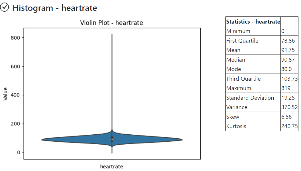
Figure 2: A sample violin plot showing probability density distribution and the summary statistics obtained from the EHR-QC exploration report giving a detailed description of the attribute

Demographics

If running via command line:

(.venv) app_user@hostname:~$python -m ehrqc.qc.Plot demographics_explore /save/path/demographics.csv /save/path/demographics_explore.html

If using Jupyter notebook:

import os

os.system(
    '''cd /path/to/EHRQC;'''
    +
    '''.venv/bin/python -m ehrqc.qc.Plot demographics_explore /save/path/demographics.csv /save/path/demographics_explore.html'''
    )

Vitals

If running via command line:

(.venv) app_user@hostname:~$python -m ehrqc.qc.Plot vitals_explore /save/path/vitals.csv /save/path/vitals_explore.html

If using Jupyter notebook:

import os

os.system(
    '''cd /path/to/EHRQC;'''
    +
    '''.venv/bin/python -m ehrqc.qc.Plot vitals_explore /save/path/vitals.csv /save/path/vitals_explore.html'''
    )

Lab Measurements

If running via command line:

(.venv) app_user@hostname:~$python -m ehrqc.qc.Plot lab_measurements_explore /save/path/lab_measurements_corrected.csv /save/path/lab_measurements_explore.html

If using Jupyter notebook:

import os

os.system(
    '''cd /path/to/EHRQC;'''
    +
    '''.venv/bin/python -m ehrqc.qc.Plot lab_measurements_explore /save/path/lab_measurements_corrected.csv /save/path/lab_measurements_explore.html'''
    )

Anomaly Reports

In addition to the all attributes summary and missing values plot that provide data overview, anomaly reports contain detail outcomes on missing analysis (Figure 3), outlier analysis (Figure 4), error analysis (Figure 5), and inconsistancies analysis (Figure 6).

Figure 3: A sample missing data analysis table from the EHR-QC anomaly report

Figure 4: A sample outlier analysis table from the EHR-QC anomaly report

Figure 5: A sample error analysis table from the EHR-QC anomaly report

Figure 6: A sample inconsistancies analysis table from the EHR-QC anomaly report

Vitals

If running via command line:

(.venv) app_user@hostname:~$python -m ehrqc.qc.Anomalies /save/path/vitals_corrected.csv /save/path/ after_vitals  -dm -do -de -di

If using Jupyter notebook:

import os

os.system(
    '''cd /path/to/EHRQC;'''
    +
    '''.venv/bin/python -m ehrqc.qc.Anomalies /save/path/vitals_corrected.csv /save/path/ after_vitals  -dm -do -de -di'''
    )

Lab Measurements

If running via command line:

(.venv) app_user@hostname:~$python -m ehrqc.qc.Anomalies /save/path/lab_measurements_corrected.csv /save/path/ after_lab_measurements -dm -do -de -di

If using Jupyter notebook:

import os

os.system(
    '''cd /path/to/EHRQC;'''
    +
    '''.venv/bin/python -m ehrqc.qc.Anomalies /save/path/lab_measurements_corrected.csv /save/path/ after_lab_measurements -dm -do -de -di'''
    )

For the rest of this section we illustrate a few use cases demonstrating the utility of this module;

Units Mix-up

The analysis of demographic data reveled a multimodal distribution within the “Height” attribute. The generated plot (Figure 7) in the demographic data exploration report clearly illustrates the overlap of two distributions. A closer examination of the value ranges within these distributions hints at the potential mix-up of two distinct units of measurement: inches and feet.

Figure 7: Histogram showing the distribution of Height attribute before unit standardisation

To preempt any downstream errors stemming from this mixed measurement scenario, we have rectified the situation to establish uniformity by executing the following commands:

import pandas as pd
df = pd.read_csv('/save/path/demographics.csv')
df.loc[df.height < 100, 'height'] = df[df.height < 100].height * 2.54
df.to_csv('/save/path/demographics_corrected.csv', index=False)

Following these adjustments, a renewed exploration report was generated (Figure 8), showcasing the successful normalisation of the “Height” attribute to a consistent unit of measurement.

Figure 8: Histogram showing the distribution of Height attribute after unit standardisation

Empty attributes

The EHR-QC data exploration reports for lab measurements reveal certain attributes that lack any recorded values (Refer Table 1), while others exhibit low overall coverage. These attributes contribute insufficient information to enhance the predictive capability of the encompassing machine learning models. Additionally, they impede the efficacy of missing value imputation algorithms.

Table 1: Coverage of all attributes in lab measurements

Attribute	Count
lactate	0
carbondioxide_blood	0
albumin	8643
glucose_urine	1377
band_form_neutrophils	5464
base_excess_in_blood	0
potassium_blood	0
ph_blood	0
chloride_serum	12142
carbondioxide_serum	0
bilirubin	10225
leukocytes_blood_auto	0
creatinine	12146
inr	11001
sodium_serum	12145
sodium_blood	0
hemoglobin	12152
ph_bodyfluid	0
platelet_count	12140
urea_nitrogen	12133
glucose_serum	12123
chloride_blood	0
oxygen	0
bicarbonate	12143
potassium_serum	12144
anion_gap	12132
leukocytes_blood_manual	12141
hematocrit	12144
aptt	10880

Consequently, in the context of this analysis, an arbitrary choice has been made to retain an attribute for subsequent analysis only if its overall coverage surpasses the threshold of 95%. Employing this criterion, slightly less than half of the total attributes, specifically 12 out of 29 (Shown in Table 2), have met the threshold and are retained for utilisation in downstream tasks using the below commands.

import pandas as pd
df = pd.read_csv('lab_measurements.csv')

df.drop('lactate', axis=1, inplace=True)
df.drop('carbondioxide_blood', axis=1, inplace=True)
df.drop('albumin', axis=1, inplace=True)
df.drop('glucose_urine', axis=1, inplace=True)
df.drop('band_form_neutrophils', axis=1, inplace=True)
df.drop('base_excess_in_blood', axis=1, inplace=True)
df.drop('potassium_blood', axis=1, inplace=True)
df.drop('ph_blood', axis=1, inplace=True)
df.drop('carbondioxide_serum', axis=1, inplace=True)
df.drop('bilirubin', axis=1, inplace=True)
df.drop('leukocytes_blood_auto', axis=1, inplace=True)
df.drop('inr', axis=1, inplace=True)
df.drop('sodium_blood', axis=1, inplace=True)
df.drop('ph_bodyfluid', axis=1, inplace=True)
df.drop('chloride_blood', axis=1, inplace=True)
df.drop('oxygen', axis=1, inplace=True)
df.drop('aptt', axis=1, inplace=True)

df.to_csv('lab_measurements_dense.csv', index=False)

Table 2: Coverage of retained attributes in lab measurements

Attribute	Count
chloride_serum	12142
creatinine	12146
sodium_serum	12145
hemoglobin	12152
platelet_count	12140
urea_nitrogen	12133
glucose_serum	12123
bicarbonate	12143
potassium_serum	12144
anion_gap	12132
leukocytes_blood_manual	12141
hematocrit	12144

Missing Value Imputation

The anomaly reports generated by EHR-QC have revealed the existence of missing values within the dataset. The report provides a breakdown of the number of missing values and their corresponding percentages for each attribute, as illustrated in the Table 3 below:

Table 3: Table showing the counts and percentage of missing value for vitals before imputation

Attribute	Missing Count	Missing Percentage
heartrate	11	0.13
sysbp	47	0.56
diabp	47	0.56
meanbp	20	0.24
resprate	9	0.11
tempc	107	1.28
spo2	24	0.29
gcseye	50	0.6
gcsverbal	57	0.68
gcsmotor	62	0.74

While certain algorithms can accommodate missing data, others require complete datasets. In cases where algorithmic handling of missing values is not viable, the EHR-QC offers a missing data imputation utility function. This function allows for the specification of the desired imputation algorithm or the automatic simulation of missingness based on the same proportion as the input data, utilising various algorithms and selecting the optimal one. Using this utility, we performed imputation to address missing values within the vitals and lab measurements using the code below. Consequently, the missing table was updated as depicted in Table 4:

If running via command line:

(.venv) app_user@hostname:~$python -m ehrqc.qc.Anomalies /save/path/vitals.csv /save/path/ vitals -cm

If using Jupyter notebook:technique

import os

os.system(
    '''cd /path/to/EHRQC;'''
    +
    '''.venv/bin/python -m ehrqc.qc.Anomalies /save/path/vitals.csv /save/path/ vitals -cm'''
    )

The above command synthetically creates a random missingness of the proportion same as that in the original data, i.e. 0.0046 and 0.0021 in the case of vitals and lab measurements respectively. On this data, it will employ different techniques including Mean Imputation, Median Imputation, KNN Imputation, MissForest Imputation, Expectation Maximisation Imputation, and Multiple Imputation to impute the missing values. The R squared score will be computed for each approach. Subsequently, the technique yielding the highest score will be selected to impute the missing values in the provided dataset. In this specific study, the MissForest method was chosen due to its superior performance for both vital signs and laboratory measurements, achieving R squared values of 0.9984 and 0.9991, respectively.

Table 4: Table showing the counts and percentage of missing value for vitals after imputation

Attribute	Missing Count	Missing Percentage
heartrate	0	0
sysbp	0	0
diabp	0	0
meanbp	0	0
resprate	0	0
tempc	0	0
spo2	0	0
gcseye	0	0
gcsverbal	0	0
gcsmotor	0	0

The missing data plots in the EHR-QC reports visualise the missingness in the data. Please refer to the provided figures (Figure 9 and Figure 10) showcasing the missing data plots before and after imputation.

Figure 9: Missing data plot before imputation

Figure 10: Missing data plot after imputation

Removal of Extreme Values (Outliers)

Another class of anomalies, which has come to our attention through the anomaly reports (see Table 5), pertains to the presence of outliers. These outliers represent extreme values that deviate significantly from the norm, rendering them inappropriate due to their eccentric nature.

Table 5: Table showing the counts and percentage of outliers for vitals before imputation

Attribute	Outlier Count	Outlier Percentage
heartrate	33	0.39
sysbp	344	4.1
diabp	179	2.13
meanbp	281	3.34
resprate	113	1.34
tempc	476	5.71
spo2	233	2.77
gcseye	0	0
gcsverbal	0	0
gcsmotor	809	9.66

These observations can disproportionately impact the predictive capabilities of Machine Learning models and thus necessitate removal. Typically, this is achieved by establishing rigid thresholds using specific statistical measures. For instance, values that surpass 2.5 times the standard deviation (SD) or 1.5 times the interquartile range (IQR) are flagged as outliers. However, we acknowledge that these predefined thresholds lack nuance and often fail to consider the domain-specific intricacies of the data. To address this limitation, EHR-QC employs a technique known as Item Response Theory (IRT) to autonomously identify extreme values. Leveraging this approach, we have implemented this feature to detect and subsequently eliminate outliers from ensuing processes using the code provided below. The effectiveness of outlier removal is clearly demonstrated in the provided figures (Figure 11 and Figure 12), showcasing the successful elimination of all potentially disruptive outliers from the dataset, ensuring they do not interfere with downstream modeling endeavors.

If running via command line:

(.venv) app_user@hostname:~$python -m ehrqc.qc.Anomalies /save/path/vitals.csv /save/path/ vitals -co

If using Jupyter notebook:

import os

os.system(
    '''cd /path/to/EHRQC;'''
    +
    '''.venv/bin/python -m ehrqc.qc.Anomalies /save/path/vitals.csv /save/path/ vitals -co'''
    )

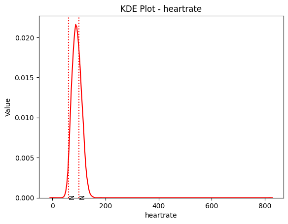
Figure 11: Distribution of heart rate before removing the outliers

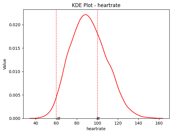
Figure 12: Distribution of heart rate after removing the outliers

7. Data Preparation

As a final step, we have used the data after correcting the anomalies (Refer Figure 13 and Table 6) to perform standardisation and normalisation using utlity functions of EHR-QC to create final data matrix. The code used to perform these operations is also provided below for reference.

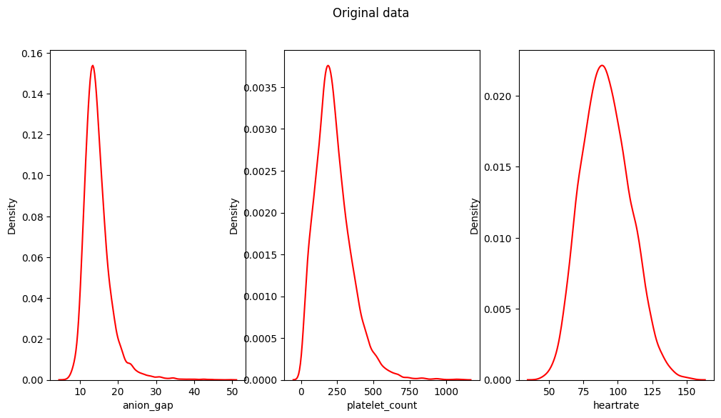
Figure 13: Distribution of heart rate without anomalies

Table 6: Table showing the summary statistics for 3 sample attributes before rescaling

Statistic	anion_gap	platelet_count	heartrate
min	6.333333	8.500000	43.354839
q1	12.400000	140.446429	78.863636
mean	14.690474	226.773821	91.543414
median	14.000000	207.666667	90.700000
mode	13.000000	168.000000	95.000000
q3	16.053933	291.541667	103.304348
max	49.285714	1110.312500	154.500000
std	3.723017	127.567722	17.318017
var	13.860854	16273.523719	299.913722

Standardisation refers to reshaping the data such that it follows a unit normal distribution with mean 0 and standard deviation 1 (Refer Figure 14 and Table 7).

If running via command line:

(.venv) app_user@hostname:~$python -m ehrqc.qc.Standardise /save/path/vitals_corrected.csv /save/path/vitals_standardised.csv

If using Jupyter notebook:

import os

os.system(
    '''cd /path/to/EHRQC;'''
    +
    '''.venv/bin/python -m ehrqc.qc.Standardise /save/path/vitals_corrected.csv /save/path/vitals_standardised.csv'''
    )

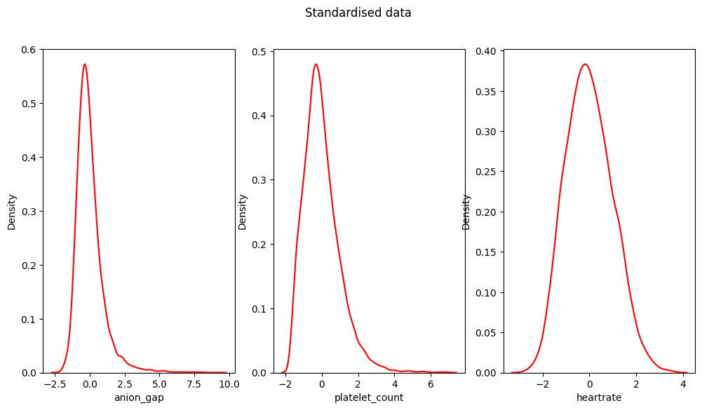
Figure 14: Distribution of heart rate after standardisation

Table 7: Table showing the summary statistics for 3 sample attributes after standardisation

Statistic	anion_gap	platelet_count	heartrate
min	-2.244846e+00	-1.711137e+00	-2.782793e+00
q1	-6.152539e-01	-6.767554e-01	-7.322315e-01
mean	-5.661282e-16	-4.299213e-17	-2.811541e-16
median	-1.854712e-01	-1.497887e-01	-4.870545e-02
mode	-4.540854e-01	-4.607518e-01	1.996108e-01
q3	3.662444e-01	5.077414e-01	6.791701e-01
max	9.292771e+00	6.926417e+00	3.635615e+00
std	1.000055e+00	1.000055e+00	1.000080e+00
var	1.000110e+00	1.000110e+00	1.000161e+00

Normalisation refers to rescaling the data such that all the values lie within a certain boundary usually between 0 and 1 (Refer Figure 15 and Table 8).

If running via command line:

(.venv) app_user@hostname:~$python -m ehrqc.qc.Rescale /save/path/vitals_corrected.csv /save/path/vitals_rescaled.csv

If using Jupyter notebook:

import os

os.system(
    '''cd /path/to/EHRQC;'''
    +
    '''.venv/bin/python -m ehrqc.qc.Rescale /save/path/vitals_corrected.csv /save/path/vitals_rescaled.csv'''
    )

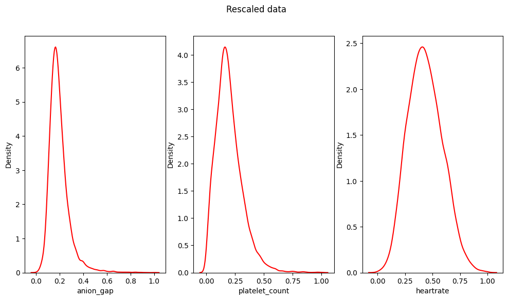
Figure 15: Distribution of heart rate after normalisation

Table 8: Table showing the summary statistics for 3 sample attributes after normalisation

Statistic	anion_gap	platelet_count	heartrate
min	0.000000	0.000000	0.000000
q1	0.141242	0.119754	0.319481
mean	0.194568	0.198104	0.433564
median	0.178492	0.180763	0.425976
mode	0.155211	0.144761	0.464664
q3	0.226311	0.256887	0.539380
max	1.000000	1.000000	1.000000
std	0.086678	0.115780	0.155814
var	0.007513	0.013405	0.024278

Note

Please note that the standardisation and normalisation is performed only on the numerical attributes and not on the categorical attributes.

8. Conclusion

In this case study, we have curated a patient cohort from a publicly accessible EHR repository. By utilising various features provided by EHR-QC, we have processed and structured this data, making it suitable for machine learning analysis. This endeavor highlights the simplicity, flexibility, versatility, diverse capabilities, utility, and practicality of EHR-QC.